
This is the second part of a series. If you haven't, you should read part 1...
Model Preparation
The text I trained the model on is available on the Gutenberg Project. Why this one? Why not?
It has a fairly varied vocabulary and a consistency of grammar and phrase structures that should trigger the model. One of the main problems of picking the wrong corpus is that it leads to cycles in the prediction with the most common words, e.g. "and the most and the most and the most and the" because it's the pattern that you see most in the text. Tacitus, at least, should not have such repetitive turns of phrase. And it's interesting in and of itself, even though it's a bit racist, or more accurately, elitist. 😂
One of the difficult decisions is choosing the type of network we will be trying to train. I tend to have fairly decent results with RNNs on that category of problems so that's what I'll use. The types and sizes of these matrices is wayyyyy beyond the scope of this piece, but RNNs tend to be decent generalists. Two RNN/LSTM layers of 512 hidden nodes will give me enough flexibility for the task and good accuracy.
What are those and how do they work? You can do a deep dive on LSTM and RNN on Wikipedia, but the short version is, they work well with sequences because the order of the input is in and of itself one of the features it deals with. Recommended for handwriting recognition, speech recognition, or pattern analysis.
Why two layers? The way you "nudge" parameters in the training phase means that you should have as many layers as you think there are orders of things in your dataset. In the case of text pattern recognition, you can say that what matters is the first order of recognition (say, purely statistical "if this word then this word") or you can add a second order where you try to identify words that tend to have similar roles in the structure (e.g. subject verb object) and take that into account as well. Higher orders than that, in this particular instance, have very little meaning unless you are dealing with, say, a multilingual analysis.
That's totally malarkey when you look at the actual equations, but it helps to see it that way. Remember that you deal with probabilities, and that the reasoning the machine will learn is completely alien to us. By incorporating orders in the model, you make a suggestion to the algorithm, but you can't guarantee that it will take that route. It makes me feel better, so I use it.
Speaking of layers, it is another one of these metaphors that help us get a handle of things, by organizing our code and the way the algorithm treats the data.
You have an input, it will go through a first layer of probabilities, then a second layer will take the output of the first one, and apply its probabilities, and then you have an output.
Let's look at the actual contents of these things:
- Input is a list of trigrams associated with a word (
(borrowing a warrant) -> from,(his father Laertes) -> added, etc - The first layer has a single input (the trigram), and a function with 512 tweakable parameters to output the label
- The second layer is trickier: it takes the 512 parameters of the first layer, and has 512 tweakable parameters of its own, to deal with the "higher order" of the data
It sounds weird, but it works, trust me for now, you'll experiment later.
The very first step is "reshaping" the trigrams so that LSTM can deal with it. We basically turn the matrices around and chunk them so that they are fed to the model as single inputs, 3 of them, in this order. It is actually a layer of its own called Reshape.
And finally, we need to write that using this model requires these steps:
- reshape
- rnn1
- rnn2
- get something usable out of it
The code, then the comments:
struct TextModel : Layer {
    @noDerivative var inputs : Int
    @noDerivative var hidden : Int
    var reshape : Reshape<Float>

    var rnn1 : RNN<LSTMCell<Float>>
    var rnn2 : RNN<LSTMCell<Float>>

    var weightsOut : Tensor<Float> {
        didSet { correction = weightsOut+biasesOut }
    }
    var biasesOut : Tensor<Float> {
        didSet { correction = weightsOut+biasesOut }
    }
    fileprivate var correction: Tensor<Float>

    init(input: Int, hidden: Int, output: Int, weights: Tensor<Float>, biases: Tensor<Float>) {
        inputs = input
        self.hidden = hidden
        reshape = Reshape<Float>([-1, input])

        let lstm1 = LSTMCell<Float>(inputSize: 1, hiddenSize: hidden)
        let lstm2 = LSTMCell<Float>(inputSize: hidden, hiddenSize: hidden)
        rnn1 = RNN(lstm1)
        rnn2 = RNN(lstm2)

        weightsOut = weights
        biasesOut = biases
        correction = weights+biases
    }

    @differentiable
    func runThrough(_ input: Tensor<Float>) -> Tensor<Float> {
        let reshaped = reshape.callAsFunction(input).split(count: inputs, alongAxis: 1)
        let step1 = rnn1.callAsFunction(reshaped).differentiableMap({ $0.cell })
        let step2 = rnn2.callAsFunction(step1).differentiableMap({ $0.cell })
        let last = withoutDerivative(at:step2[0])
        let red = step2.differentiableReduce(last, { (p,e) -> Tensor<Float> in return e })
        return red
    }

    @differentiable
    func callAsFunction(_ input: Tensor<Float>) -> Tensor<Float> {
        let step2out = runThrough(input)
        let step3 = matmul(step2out, correction)
        return step3
    }
}
The RNN/LTSM have been talked about, but what are these two functions?
callAsFunction is the only one needed. I have just decided to split the algorithm in two: the part where I "just" pass through layers, and the part where I format the output. Everything in runThrough could be written at the top of callAsFunction.
We follow the steps outlined previously, it all seems logical, even if the details aren't quite clear yet.
What is it with the @noDerivative and @differentiable annotations?
Because we are dealing with a structure (model, layer, etc...) that not only should but will be adjusted over time, it is a way to tell the system which parts are important to that adjustment:
- all properties except those maked as not derivative will be nudged potentially, so it makes sense to mark the number of inputs as immutable, and the rest as "nudgeable"
- all the functions that calculate something that will be used in the "nudging" need to have specific maths properties that make the change non-random. We need to know where we are and where we were going. We need a position, and a speed, we need a value and its derivative
Ugh, maths.
Yeah.
I am obviously oversimplifying everything to avoid scaring away everyone from the get go, but the idea should make sense if you look at it this way:
- Let's take a blind man trying to shoot an arrow at a target
- You ask them to shoot and then you'll correct them based on where the arrow lands
- It hits the far left of the target
- You tell them to nudge the aim to the right
- The problem is that "more right" isn't enough information... You need to tell them to the right a little (new position and some information useful for later, you'll see)
- The arrow lands slightly to the right of the center
- You tell the archer to aim to the left but less than their movement they just made to the right.
Two pieces of information: one relative to a direction, and one relative to the rate of change. The other name of the rate of change is the derivative.
Standard derivatives are speed to position (we are here, now we are there, and finally we are there, and the rate of change slowed, so the next position won't be as far from this one as the one was to the previous one), or acceleration to speed (when moving, if your speed goes up and up and up, you have a positive rate of change, you accelerate).
That's why passing through a layer should preserve the two: the actual values, and the speed at which we are changing them. Hence the @differentiable annotation.
(NB for all you specialists in the field reading that piece... yes I know. I'm trying to make things more palatable)
"But wait", say the most eagle-eyed among you, "I can see a withoutDerivative in that code!"
Yes. RNN is peculiar in the way that it doesn't try to coerce the dimensions of the results. It spits out all the possible variants it has calculated. But in practice, we need only the last one. Taking one possible outcome out of many cancels out the @differentiable nature of the function, because we actually lose some information.
This is why we only partially count on the RNN's hidden parameters to give us a "good enough" result, and need to incorporate extra weights and biases that are derivable.
The two parts of the correction matrix, will retain the nudge speed, as well as reshape the output matrix to match the labels: matrix addition and multiplications are a bit beyond the scope here as well (and quite frankly a bit boring), but that last step ( step3 in the code ) basically transform a 512x512x<number of labels> matrix, into a 2x<numbers of labels> : one column to give us the final probabilities, one for each possible label.
If you've made it this far, congratulations, you've been through the hardest.
Model Training
OK, we have the model we want to use to represent the various orders in the data, how do we train it?
To continue with the blind archer metaphor, we need the piece of code that acts as the "corrector". In ML, it's called the optimizer. We need to give it what the archer is trying to do, and a way to measure how far off the mark the archer is, and a sense of how stern it should be (do we do a lot of small corrections, or fewer large ones?)
The measure of the distance is called the "cost" function, or the "accuracy" function. Depending on how we look at it we want to make the cost (or error) as low as possible, and the accuracy as high as possible. They are obviously linked, but can be expressed in different units ("you are 3 centimeters off" and "you are closer by 1%"). Generally, loss has little to no meaning outside of the context of the layers ( is 6 far? close? because words aren't sorted in any meaningful way, we are 6.2 words away from the ideal word doesn't mean much), while accuracy is more like a satisfaction percentage (we are 93% satisfied with the result, whatever that means).
func accuracy(predictions: Tensor<Int32>, truths: Tensor<Int32>) -> Float {
    return Tensor<Float>(predictions .== truths).mean().scalarized()
}

let predictions = model(aBunchOfFeatures)
print("Accuracy: \(accuracy(predictions: predictions.argmax(squeezingAxis: 1), truths: aBunchOfLabels))")
Accuracy: 0.10143079
and the loss:
let predictions = model(aBunchOfFeatures)
let loss = softmaxCrossEntropy(logits: predictions, labels: aBunchOfLabels)
print("Loss test: \(loss)")
Loss test: 6.8377414
In more human terms, the best prediction we have is 10% satisfying, because the result is 6.8 words away from the right one. 😬
Now that we know how to measure how far off the mark we are (in two different ways), we need to make a decision about 3 things:
- Which kind of optimizer we want to use (we'll use
Adam, it's a good algorithm for our problem, but other ones exist. For our archer metaphor, it's a gentle but firm voice on the corrections, rather than a barking one that might progress rapidly at first then annoy the hell out of the archer) - What learning rate we want to use (do we correct a lot of times in tiny increments, or in bigger increments that take overall less time, but might overcorrect)
- How many tries we give the system to get as close as possible
You can obviously see why the two last parameters are hugely important, and very hard to figure out. For some problems, it might be better to use big steps in case we find ourselves stuck, for others it might be better to always get closer to the target but by smaller and smaller increments. It's an art, honestly.
Here, I've used a learning rate of 0.001 (tiny) and a number of tries of 500 (medium), because if there is no way to figure out the structure of the text, I want to know it fast (fewer steps), but I do NOT want to overshoot(small learning rate).
Let's setup the model, the correction matrices, and the training loop:
var weigths = Tensor<Float>(randomNormal: [512, contents.vocabulary.count]) // random probabilities
var biases = Tensor<Float>(randomNormal: [contents.vocabulary.count]) // random bias
var model = TextModel(input:3, hidden: 512, output: contents.vocabulary.count, weights: weigths, biases: biases)
Now let's setup the training loop and run it:
let epochCount = 500
var trainAccuracyResults: [Float] = []
var trainLossResults: [Float] = []

var randomSampleSize = contents.original.count/15
var randomSampleCount = contents.original.count / randomSampleSize

print("Doing \(randomSampleCount) samples per epoch")
for epoch in 1...epochCount {
    var epochLoss: Float = 0
    var epochAccuracy: Float = 0
    var batchCount: Int = 0

    for training in contents.randomSample(splits: randomSampleCount) {
        let (sampleFeatures,sampleLabels) = training
        let (loss, grad) = model.valueWithGradient { (model: TextModel) -> Tensor<Float> in
            let logits = model(sampleFeatures)
            return softmaxCrossEntropy(logits: logits, labels: sampleLabels)
        }
        optimizer.update(&model, along: grad)

        let logits = model(sampleFeatures)
        epochAccuracy += accuracy(predictions: logits.argmax(squeezingAxis: 1), truths: sampleLabels)
        epochLoss += loss.scalarized()
        batchCount += 1
    }
    epochAccuracy /= Float(batchCount)
    epochLoss /= Float(batchCount)
    trainAccuracyResults.append(epochAccuracy)
    trainLossResults.append(epochLoss)
    if epoch % 10 == 0 {
       print("avg time per epoch: \(t.averageDeltaHumanReadable)")
       print("Epoch \(epoch): Loss: \(epochLoss), Accuracy: \(epochAccuracy)")
    }
}
A little bit of explanation:
- We will try 500 times (
epochCount) - At each epoch, I want to test and nudge for 15 different combinations of trigrams. Why? because it avoids the trap of optimizing for some specific turns of phrase
- We apply the model to the sample, calculate the loss, and the derivative, and update the model with where we calculate we should go next
What does that give us?
Doing 15 samples per epoch
Epoch 10: Loss: 6.8377414, Accuracy: 0.10143079
Epoch 20: Loss: 6.569199, Accuracy: 0.10564535
Epoch 30: Loss: 6.412607, Accuracy: 0.10802801
Epoch 40: Loss: 6.2550464, Accuracy: 0.10751916
Epoch 50: Loss: 6.0366735, Accuracy: 0.11123683
...
Epoch 490: Loss: 1.1177399, Accuracy: 0.73812264
Epoch 500: Loss: 0.5172857, Accuracy: 0.86724746
We like to keep these values in an array to graph them. What does it look like?
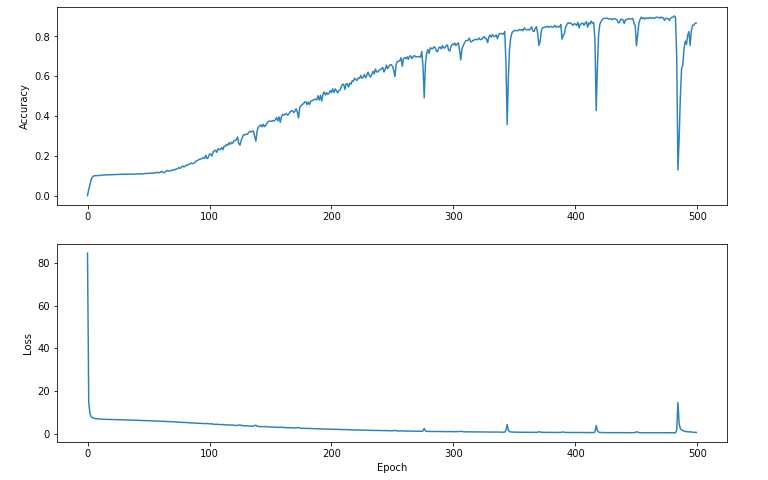
We can see that despite the dips and spikes, because we change the samples often and don't try any radical movement, we tend to better and better results. We don't get stuck in a ditch.
Next part, we'll see how to use the model. Here's a little spoiler: I asked it to generate some random text:
on flocks settlement or their enter the earth; their only hope in their arrows, which for want of it, with a thorn. and distinction of their nature, that in the same yoke are also chosen their chiefs or rulers, such as administer justice in their villages and by superstitious awe in times of old.It's definitely gibberish when you look closely, but from a distance it looks kind of okayish for a program that learned to speak entirely from scratch, based on a 10k words essay written by fricking Tacitus.